Testing a Rule Change Before Deploy with Impact Simulation

The problem

A rule change can be one character on the screen and five figures in the ledger.

Marketing asks to raise the new-customer welcome discount from 10% to 15%. In the codebase that is a single constant — 0.10 becomes 0.15. It compiles, the unit tests stay green, and the change ships on a Tuesday afternoon.

Three weeks later finance reconciles the month and finds a margin hole. The welcome discount cost more than its budget allowed. The one-character change had a blast radius nobody measured: it applied to every new-customer order for three weeks, and the extra five points compounded across a volume no one looked at before the change went live.

Nothing was wrong with the code. The constant was correct. What was missing was the answer to a question the code cannot answer on its own — across last month's orders, what would this change have cost? That question is about aggregate behavior over real data, and a constant in a service has no way to surface it before deploy.

The question this pattern answers: how does a team measure the full impact of a rule change against real historical orders before it reaches production, and decide on that evidence whether to ship.

The naive approach

The first version keeps the discount as a constant and changes it in place.

public BigDecimal applyWelcomeDiscount(Order order, Customer customer) {
    BigDecimal subtotal = order.getSubtotal();

    // Welcome discount for new customers.
    // Marketing asked to raise this from 0.10 to 0.15.
    if (customer.getSegment() == Segment.NEW) {
        BigDecimal rate = new BigDecimal("0.15"); // was 0.10
        return subtotal.subtract(subtotal.multiply(rate));
    }
    return subtotal;
}

The diff is one line, and it is the kind of change that feels too small to need a process. That feeling is the trap. The problem is not correctness — the new rate is applied correctly to every matching order. The problem is that the change ships without anyone sizing it, and that shows up in three places.

• Unit tests prove the wrong thing. A test asserts that a $100 new-customer order returns $85. It is green and it is useless for this decision, because it checks one case, not the aggregate. No test in the suite answers "what does 0.15 do to last month's 40,000 orders." The number that decides this change is not one the suite can produce.
• The blast radius is invisible until production is the test. The first real measurement of the change is the finance reconciliation weeks later. Production becomes the place you find out, and the feedback loop is a month long.
• There is no record of the decision. When finance asks why the welcome discount overran, the answer is git blame on a constant and a memory of a Slack thread. The rate that was live on any given day, and the impact it had, were never written down anywhere you can query.

Defining the pattern

The fix is to make the change something you can measure before it ships. Model the discount as a rule, treat the proposed change as a separate version, and keep the current and proposed versions side by side.

The welcome discount then sits in three LexQ objects.

• Fact: what the checkout call reports about an order. customerSegment, purchaseSubtotalUsd.
• Rule: one rule for the welcome discount — a condition and a MUTATE_FACT action that subtracts a percentage from purchaseSubtotalUsd.
• Version: an immutable snapshot of all rules. The baseline is the current production version holding the live 10% rule; the candidate — the Target Version, in the console's terms — holds the proposed 15% rule. Nothing about the candidate touches production until you deploy it.

The rule itself is ordinary. There is no mutex group here, because nothing competes — a single discount either applies to an order or it does not. When several discounts can claim the same order, that competition is its own problem, and resolving VIP tier discount stacking is where it gets settled.

{
  "name": "Welcome discount: new customers 15%",
  "condition": {
    "type": "GROUP",
    "operator": "AND",
    "children": [
      {
        "type": "SINGLE",
        "field": "customerSegment",
        "operator": "EQUALS",
        "value": "NEW",
        "valueType": "STRING"
      }
    ]
  },
  "actions": [
    {
      "type": "MUTATE_FACT",
      "parameters": {
        "operand": 15,
        "method": "PERCENTAGE",
        "targetVar": "purchaseSubtotalUsd",
        "operator": "SUB",
        "rounding": { "mode": "HALF_UP", "scale": 2 }
      }
    }
  ],
  "isEnabled": true
}

The baseline is identical except operand is 10. Duplicate the live version — the API verb is clone — change the one rule, and you have a candidate. The candidate is a real version with its own ID, so you can run anything against it, but it carries no traffic until you deploy it.

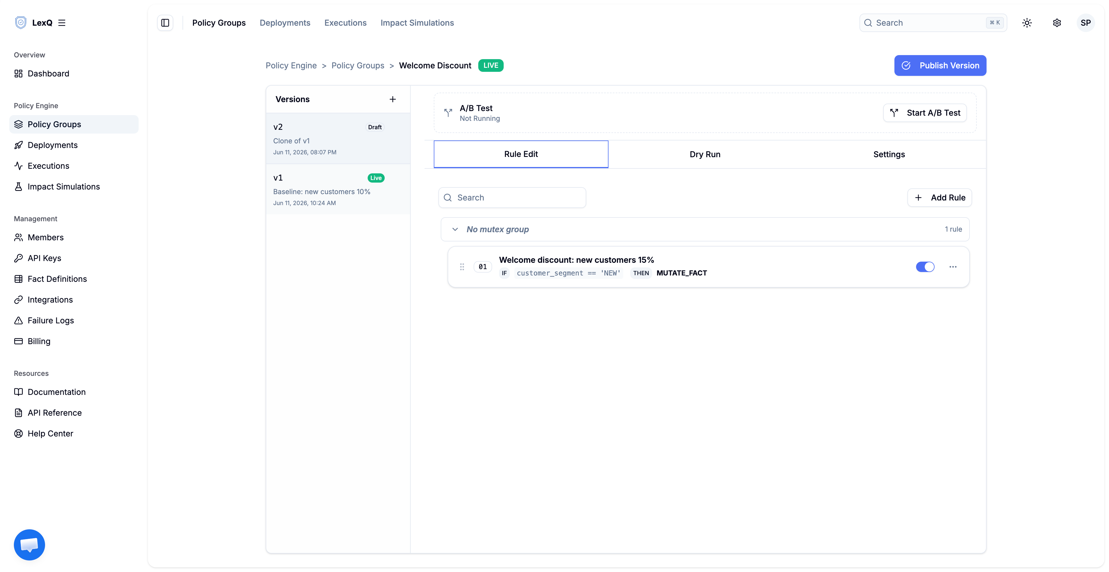
This is the setup Impact Simulation needs: two versions that differ by exactly the change you are evaluating.

Impact Simulation strategy

Impact Simulation answers the question the unit tests could not — across real orders, what does the candidate do that the baseline did not. You point it at a slice of historical execution data and run the candidate against it, with the baseline as the comparison.

The dataset is historical execution data, the real orders the engine has already processed, covering a window long enough to be representative. A full past month is a reasonable default. Each record carries the facts a real order sent (customerSegment, purchaseSubtotalUsd), so the run reproduces what would have happened on that traffic under the candidate.

lexq analytics simulation start --json '{
  "policyVersionId": "<candidate-version-id>",
  "dataset": {
    "type": "HISTORICAL",
    "source": "EXECUTION_LOGS",
    "from": "2026-05-01",
    "to": "2026-05-31"
  },
  "options": {
    "baselinePolicyVersionId": "<baseline-version-id>",
    "includeRuleStats": true,
    "maxRecords": 40000,
    "metricConfig": {
      "targetVariable": "purchaseSubtotalUsd__delta",
      "aggregationType": "SUM"
    }
  }
}'

The run replays every record through both versions and reports three things this decision turns on.

• The aggregate metric. metricConfig sums purchaseSubtotalUsd__delta across the dataset for each version. Each order's __delta is the discount that order received (a negative number); the sum is the total discount given. The candidate's sum minus the baseline's sum is the additional discount the rate change would have cost last month — the blast radius, in dollars, before deploy.
• The match rate. With includeRuleStats, the run reports how often the welcome rule fired. That rate is the share of orders from new customers. If it comes back far higher than the business expects, the customerSegment fact the application sends is suspect, and that is worth knowing before, not after.
• Baseline against candidate, side by side. The console shows both versions' numbers in one view, so the difference is read directly rather than computed by hand.

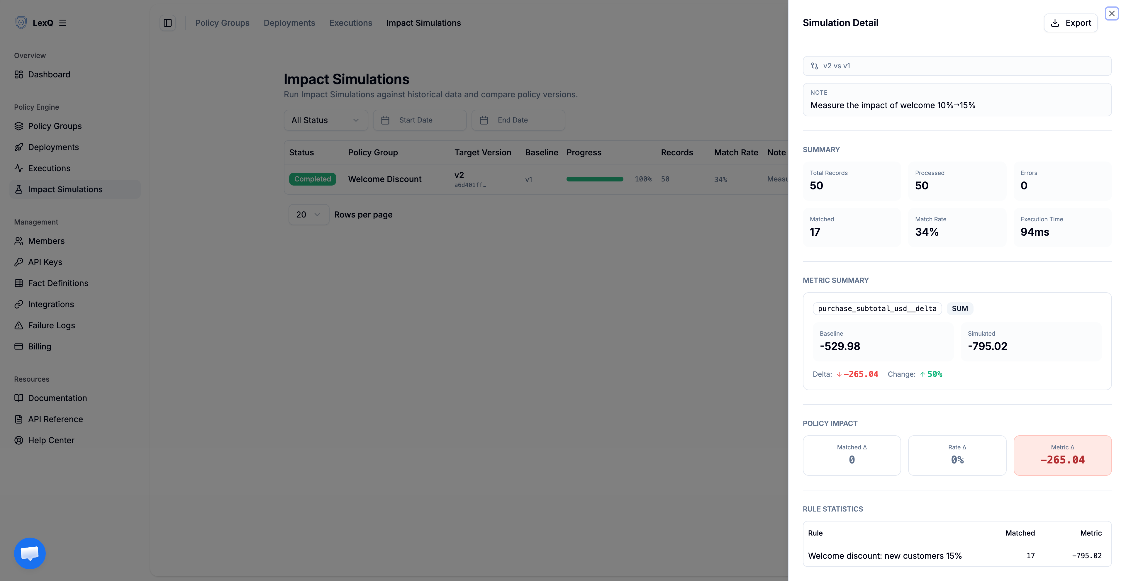
Two conditions decide whether to ship. First, the additional aggregate discount — the candidate's summed __delta minus the baseline's — must land within the budget the team set for the new-customer discount. If the simulation says the change costs more than that, the decision is made before a single live order is affected. Second, the match rate must match the expected share of new-customer orders; a large gap means the facts in production do not look like the facts you assumed. A simulation reads historical data and writes nothing. It has no side effects.

If you have no production traffic yet, upload a representative dataset instead — orders spanning new and returning segments across the subtotal range you expect — and run the same comparison against it.

Decision Trace output

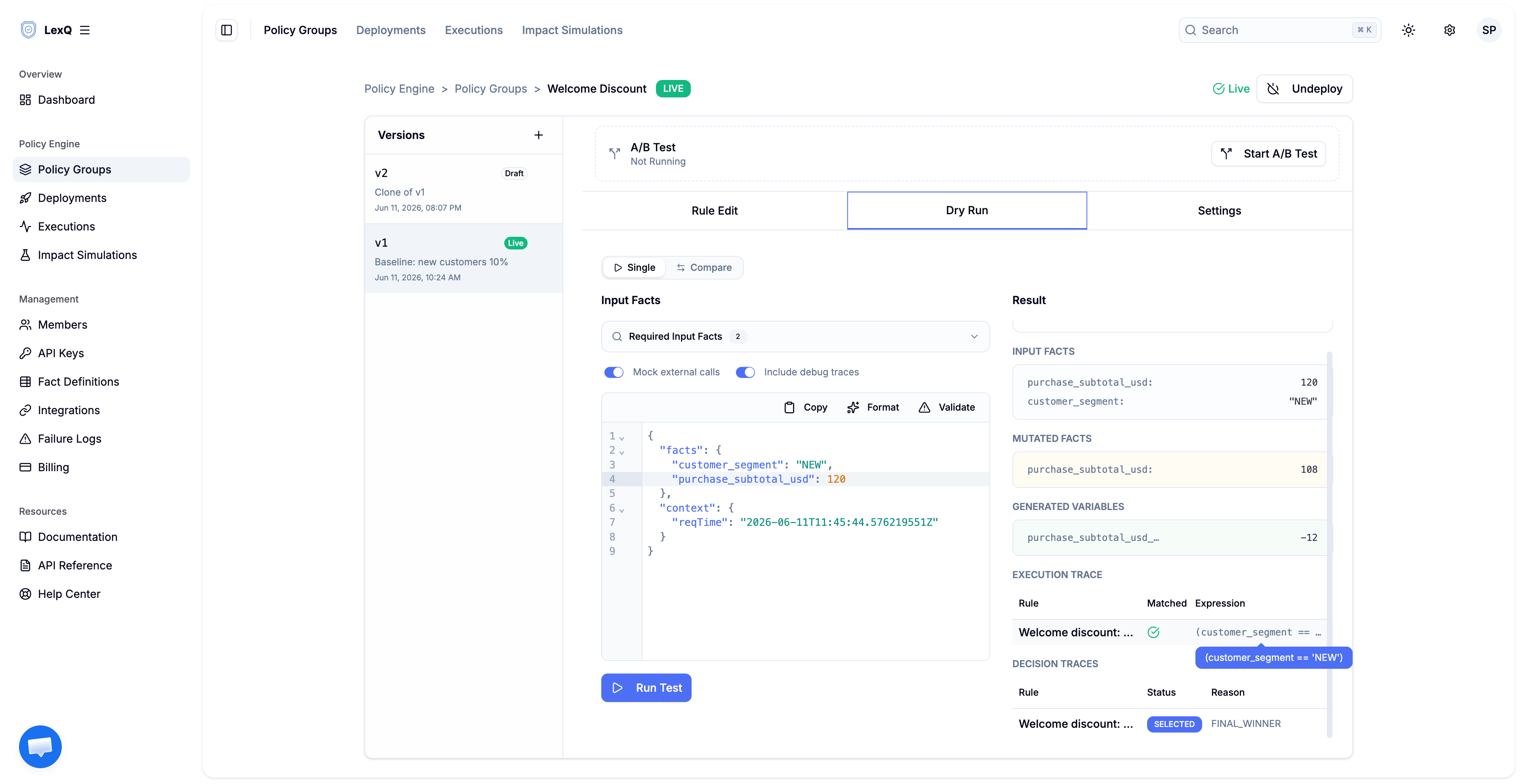
The aggregate number is built from individual decisions, and each one is inspectable. Run a single order, a new customer with a $120 cart, against the candidate with Dry Run.

{
  "result": "SUCCESS",
  "data": {
    "inputFacts": {
      "customerSegment": "NEW",
      "purchaseSubtotalUsd": 120.00
    },
    "mutatedFacts": {
      "purchaseSubtotalUsd": 102.00
    },
    "generatedVariables": {
      "purchaseSubtotalUsd__delta": -18.00
    },
    "executionTraces": [ ... ],
    "decisionTraces": [
      {
        "ruleName": "Welcome discount: new customers 15%",
        "status": "SELECTED",
        "reasonCode": "FINAL_WINNER",
        "reasonDetail": null
      }
    ]
  }
}

mutatedFacts holds the discounted subtotal, 102.00. generatedVariables carries purchaseSubtotalUsd__delta, -18.00 — exactly 15% of 120, and exactly the amount this one order contributes to the aggregate the simulation summed. The relationship is direct: the dollar figure in the simulation is the sum of these per-order deltas. In decisionTraces, the welcome rule is SELECTED with reasonCode FINAL_WINNER; the expression it was evaluated against appears in the Execution Trace table in the Dry Run view above. Six months on, the $18 taken off this order is explained by the stored trace, not by attaching a debugger to a running service.

Run the same order through the baseline (the 10% version) and the delta is -12.00, the subtotal 108.00. The $6 gap on this one order is 5% of its subtotal, and the same 5% comes off every matching order; summed across the month, that is the additional cost the simulation reported in aggregate. A returning customer's order matches no rule at all — status NO_MATCH, reasonCode CONDITION_MISMATCH — and carries no discount under either version, which is why the match rate, not just the rate value, moves the aggregate.

Edge cases

The pattern is the simulation workflow, not the discount. The choices below decide whether the simulated number is worth trusting.

• Choosing the metric. SUM of purchaseSubtotalUsd__delta answers "total discount given." Other questions need a different metricConfig. AVG answers "average discount per discounted order" — it divides by the orders that carry a __delta under both versions, not by every order in the dataset, because an order no rule touched has no such key to average. "How many orders were affected" is read from the change distribution, which counts the records whose value moved. Pick the aggregation that matches the question you are actually asking, and confirm the sign — for a discount the delta is negative, so a larger discount is a more negative sum.
• Non-deterministic rules. A rule whose outcome depends on wall-clock time or a random draw will not replay identically, because the historical record captured one roll of that input. Keep the facts a rule reads explicit and deterministic. If a rule genuinely depends on time, simulate within a window where that dependency is stable.
• A representative dataset, not a tidy one. When you upload data instead of replaying production, the temptation is to include only clean cases. The cases that move the aggregate are the ones at the edges — the largest carts, the segment boundaries. A dataset without them produces a number that looks safe and is not.
• Sample size. maxRecords caps the run. A cap small enough to miss a rare high-value segment gives a confident answer about the wrong population. Size the window and the cap to cover the volume the change will actually touch.
• The simulation is read-only. Rule actions change facts and record decisions, so nothing leaves the engine and the run writes nothing back. The aggregate is computed without any external effect, which is what makes it safe to run against a full month repeatedly.

Production rollout

The 15% version goes live through Deploy once the cost figure and the match rate both pass. The deploy seals that rule snapshot under a hash, verifies its integrity, and files who shipped 15% and when. To expose the change gradually instead of cutting all traffic over at once, run an A/B test between the candidate and the current live version and raise the candidate's traffic share in steps — 5% → 25% → 50%. At each step you watch the live decision traces and the running aggregate, and only advance if the live numbers track the simulation; when they hold, deploy the candidate to take over the remaining traffic.

Two readings on live traffic call for an immediate rollback:

• The live aggregate discount drifts from the simulation's prediction as traffic ramps. The production population differs from the historical window you simulated against, and the blast radius you signed off on no longer holds.
• The welcome rule fires at a rate far from the simulation's match rate. The customerSegment fact the application sends in production does not match what the dataset contained.

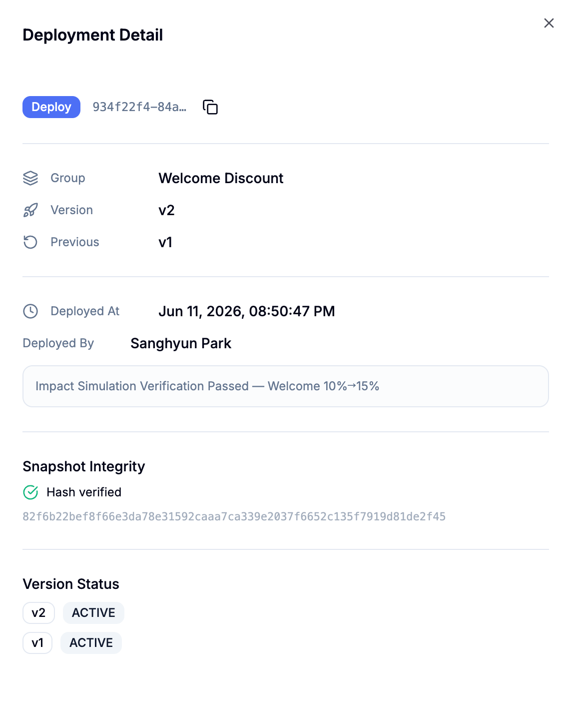
Rolling back re-points the policy group at the 10% version, and it writes its own deployment record, so the return to 10% is as traceable as the move to 15%. Once the candidate is serving all traffic, the rule statistics show the welcome rule's live match rate and the realized aggregate — the same two numbers the simulation predicted, now measured. The gap between predicted and realized is the calibration you carry into the next change. If checkout slows down once the 15% version carries all traffic, the next question is which rule spent the milliseconds. Isolating a slow rule on a hot path answers it with per-rule timings.

---

See how LexQ works for yourself in the playground.